


Economic Summary
Construction
Construction Spending rose 0.5% in October compared to a 0.6% decline in September. Residential construction spending accounted for all the increase as it increased 1.0% while nonresidential spending was unchanged from September.
Consumer Sentiment
Consumers came out of the holiday season in a more optimistic mood. The University of Michigan Consumer Sentiment index rose from 52.9 in December to 56.4 in January. The improvement occurred in both sub-indices. The Current Conditions sub-index rose from 50.5 to 55.4 while the Future Expectations sub-index rose from 54.6 to 57.0.
Economic Growth
The Bureau of Labor Statistics revised 3rd quarter economic growth from the originally reported 4.3% annualized growth to 4.4%.
Housing
Mortgage applications experienced another strong week of activity as mortgage applications rose 14.4% last week after rising 28.5% the week before. Perhaps consumers are not convinced the decline in mortgage rates will last and are trying to lock in their rates now. Applications to purchase a home rose 5.1% while applications to refinance rose 20.4%. The average 30-year mortgage rate was essentially unchanged at 6.16% compared to 6.18% the week before. After rising 3.3% in November, pending home sales declined 9.3% in December.
Inflation
The pace of inflation increased in November when measured by the Personal Consumption Expenditures (PCE) Price Index. The PCE Price Index rose 2.8% on a year-over-year basis after rising at a 2.7% pace in September (October was not calculated due to the government shutdown). The Core PCE Price Index also rose 2.8% after rising 2.7% in September.
Jobs
Initial Jobless Claims fell 1,000 last week and totaled 200,000. Continuing claims fell 26,000 to 1,849,000.
Manufacturing Activity
S&P Global's Manufacturing PMI showed minor improvement in January. The index rose from 51.8 in December to 51.9 in January.
Personal Income
Personal income rose 4.3% on a year-over-year basis in November. Personal income after taxes and inflation rose1.0%.
Personal Spending
Consumers continue to spend at a faster pace than their income growth. Personal spending rose 5.4% and rose 2.6% after inflation.
Service Sector Activity
S&P Global's Service Sector PMI was unchanged in January compared to December. The index remained at 52.5.
Perspectives
Affordability has been the hot topic in the political arena as mid-term election campaigning kicks into full gear. One of the biggest areas of concern when it comes to affordability is housing affordability. This week's Perspectives examines housing affordability at the state level.
Soundbite
The ability for the average individual in the US to qualify for a 30-year mortgage to buy a house is now becoming an option only available to the upper income individuals. There are only 8 out of the 50 states (16%) where the expense-to-personal income ratio to qualify for a conventional 30-year mortgage meets the maximum 28% level established by most mortgage lenders. That assumes that the average person in the state has all the income sources used to calculate the state's average personal income. The situation becomes worse if you remove some of the income sources that middle-or lower-income individuals do not traditionally have. This means that for most households to be able to buy a house, they need two individuals with all the income sources to qualify for house. Under that scenario, the ratio jumps from 16% of the states to 96%. The problem with that solution is if something happens to one of the income sources (i.e., reduced hours or job loss). That situation would force the household to divert a large part of their income to their mortgage payment and dramatically reduce spending in all other categories.
The dramatic increase in home prices over the last 5 to 10 years has been a driving force in the affordability problem. Increased taxes and insurance costs exacerbate the problem. From an economic perspective, the way to stabilize or reduce prices is for supply of homes to increase or demand for homes to decrease. That is far easier said than done.
Analysis
For most households that want to buy a house, the goal/dream is to qualify for a mortgage using only one of the income earner's income. This would then allow the second income earner's income to be used to pay for all the other family expenses (i.e., groceries, utilities, healthcare, daycare, college savings, etc.). As a result, this analysis will examine affordability using one income earner's income.
Besides your credit rating, the most important hurdle to clear to qualify for a mortgage is meeting the expense to income ratio for the mortgage. Mortgage lenders include four components to calculate the expenses related to the mortgage: mortgage payment (principal and interest), property tax, and insurance on the house. This is called PITI. They will then calculate the PITI to Gross Income ratio. Gross income sweeps in all income sources: wages or salaries, business owner's income, interest income, dividends, and transfer payments. In general, most conforming mortgages are financed using one of three government agency guarantee programs: GNMA, FNMA and FHLMC. These programs set a maximum threshold for the PITI/Income ratio at 28%. Loans guaranteed by USDA allow a PITI/Income ratio as high as 29% and FHA/VA will go as high as 31%. Naturally, there are exceptions and there are sometimes first-time home buyer programs that may accept a higher ratio.
Let us start by examining the top and bottom 10 states for PITI/Income ratios using one wage earner's gross income. The first graph below shows is that there are only 8 out of the 50 states (16%) where a single income earner's total income would result in a PITI/Income ratio that would be 28% or lower. If we apply the 29% USDA limit, 10 (20%) and there are 16 states (32%) would meet the USDA limit of 31%.
Hawaii is that state with the highest PITI/Income ratio and, as the lower chart shows, 9 out of the bottom 10 states have a PITI/Income ratio at 50% or more. The three states where Washington Trust Bank has offices all have expense-to-income ratios at or above 50%. A side note is that Idaho ranked as an affordable state 10 years ago, but as the state became identified as an affordable place to live, people started to move from the expensive states to Idaho. Even though this has benefited Idaho from a population and labor pool standpoint it created the negative result of increased demand outstripping supply and driving home price dramatically higher. Now Idaho has the dubious honor of being the sixth most unaffordable state from a housing perspective. The problem is Idaho's per capita personal income is below the US, but its average home price is above the US average.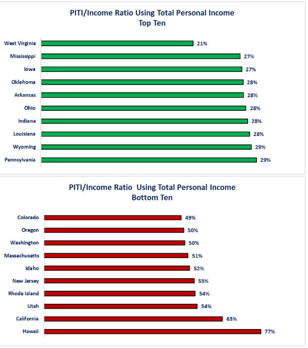
At a state level, all income sources exist to calculate the per capita personal income for the state. The reality is that not all individuals in the state have all those income sources. Business owner's income is limited to someone who owns a business. Interest and dividends are mostly limited to higher income individuals. If we want to gain perspective on the ability for middle and lower-income households to buy a house, we can exclude the above income sources in the calculation. Let us examine how many states would have an expense-to-income ratio below 31% if we exclude business owner's income, dividends, and income. The first chart below shows that only one state (2%) would meet the 28% threshold and no additional states would qualify if we used the 29% and 31% ratios. 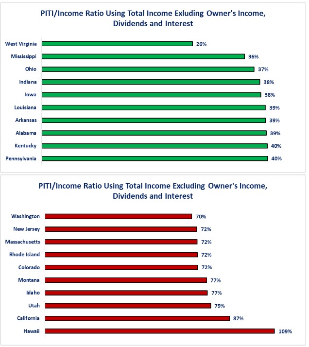
Finally, let us take it one step further to see the impact on a household who only has their wages or salary. This analysis excludes business owner's income, interest, dividends, and transfer payments. It also examines net wages or salaries (after payroll tax deductions). This is clearly the most extreme scenario from an income perspective, but the reality is that, for many first time home buyers, that is their income situation. As the first chart below illustrates, for this type of for household, the prospect of buying a house using one income earner's income is a distant pipe dream. The best state in this scenario has an expense-to-income ratio of 59%. The second graph illustrates that the 10 least affordable states would have expense-to income ratios between 115% to 196%.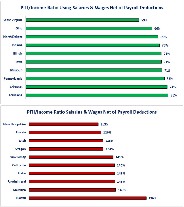
The implications from the information provided above is that buying a house using one income earner's income is only available to upper income households. For the rest, buying a house requires two income earners. Assuming the two income earners in a household both have incomes that match the per capita income of a state, the picture dramatically changes.
-
Assuming the per capita income for the state for two income earners, 96% of states would then have an expense-to-income ratio below 28%. The number does not change using 29% or 31% as the last two states (California and Hawaii) are above those levels.
-
Excluding business owner's income, dividends, and interest, 34 out 50 states (68%) would have an expense-to-income ratio below 28%. Once again, the percentage does not change using 29% and 31% as the 35th state's ratio is above either of these levels.
-
Using the net wage or salary income does not show any state meeting the 28% level, but it does result in one state (West Virginia) meeting the 31% qualifying level.
Conclusions
Given the data reviewed above, it is clear that housing affordability is a national problem. The reality though, is that it requires local solutions as there is no “one size fits all” solution from a national level.
For some states (and municipalities) the primary problem lies squarely in a lack of supply compared to the demand for housing.
For other states, it is an income problem as the type of businesses that are fueling jobs growth in a state may not have wages or salaries that can offset the home price and related expenses.
For other states, their housing policies and procedures result in the types of homes desired from home buyers not being profitable to build.
Lastly, it is likely that the problem is a combination or all the above.
From an economic perspective, if a state becomes highly unaffordable for the average household, the risk is that people and/or businesses move to more affordable states. This results in a direct loss of revenue for the state and potentially creates excess infrastructure that must be maintained even though the population no longer needs or uses it. That means fixed expenses, or rising expenses, without the income to offset.
Housing affordability is also a risk for states that are currently affordable. Unless there is proactive planning for how to manage or control the migration to their state, an affordable state may quickly become unaffordable due to demand outstripping supply.
Ultimately, the solution requires collaboration and cooperation between the four stakeholders. Pointing fingers or blaming one stakeholder does not create solutions.
Governments will need to find ways to ensure their policies, procedures and taxes support developing houses. One of the critical examples of this is for states to ensure that their housing policies (i.e., permitting, building codes, environmental, etc.) are consistent across the whole state. It is very hard to expect builders to reduce costs through economies of scale for building when each city and county may have a different set of policies.
Builders will need to find ways to increase efficiency and productivity to control costs for building. Whether that is new supply sources, new materials, AI, automation, robotics, 3D printing, factory production, etc. remains to seen as to which may be a viable solution.
Neighborhoods will need to realize and understand that a “not in my backyard” mentality may seem like a good solution in the short-term but increasing the cost of building via litigation and delays or preventing building may well prove to be a terrible solution for the neighborhood in the long-term as people start to leave the area due to affordability issues. Being at the table as a stakeholder to ensure new building incorporates the necessary infrastructure to avoid congestion and other problems is one thing; flat out opposing all new developments is something completely different and is not being part of the solution.
Prospective home buyers also need to have a seat at the table as a stakeholder because they can identify what type of housing they desire. If government officials, builders or neighborhoods all think that what was desired in the past is still what is desired by the next generation, then they risk a mismatch of supply versus demand. One example of this is that the younger generation may not want a yard to maintain, may not care if their house is six feet away from their neighbor (their apartment is wall to wall) and are fine with a house that is less than 1,500 square feet but local officials, builders, or neighborhoods still think that a house should be at least 2,000 square feet and sit on a ¼ acre piece of land. Without the buyer as a stakeholder, the opportunity to discuss building different houses compared to the current houses is lost.
The basic economic solution to the housing affordability issue is that either the supply of homes needs to increase or demand needs to decrease in order to stabilize or reduce housing costs. That sounds simple but, as discussed above, that is far more complex to actually achieve.
Disclosures
Personal Income: Bureau of Labor Statistics.
Home Values: Zillow Home Value Index.
Property Taxes: Tax Foundation Property Taxes by State and County.
Homeowners Insurance: Bankrate
Mortgage Payment: Assumes 30-year fixed rate mortgage, average down payment of 14.4% and 6.20% mortgage rate.
Average Down Payment: Realtor.com.

Steve is the Economist for Washington Trust Bank and holds a Chartered Financial Analyst® designation with over 40 years of economic and financial markets experience.
Throughout the Pacific Northwest, Steve is a well-known speaker on the economic conditions and the world financial markets. He also actively participates on committees within the bank to help design strategies and policies related to bank-owned investments.